数据整理

library(vegan)

## 载入需要的程辑包：permute

## 载入需要的程辑包：lattice

## This is vegan 2.6-4

data("varespec")
pca <- rda(varespec)

首先看一下结果：

summary(pca)

## 
## Call:
## rda(X = varespec) 
## 
## Partitioning of variance:
##               Inertia Proportion
## Total            1826          1
## Unconstrained    1826          1
## 
## Eigenvalues, and their contribution to the variance 
## 
## Importance of components:
##                            PC1      PC2       PC3     PC4      PC5      PC6
## Eigenvalue            982.9788 464.3040 132.25052 73.9337 48.41829 37.00937
##                            PC7      PC8       PC9      PC10     PC11     PC12
## Eigenvalue            25.72624 19.70557 12.274191 10.435361 9.350783 2.798400
##                           PC13      PC14      PC15      PC16      PC17
## Eigenvalue            2.327555 1.3917180 1.2057303 0.8147513 0.3312842
##                            PC18      PC19      PC20      PC21      PC22
## Eigenvalue            0.1866564 1.065e-01 6.362e-02 2.521e-02 1.652e-02
##                            PC23
## Eigenvalue            4.590e-03
## [到达getOption("max.print") -- 略过2行]]
## 
## Scaling 2 for species and site scores
## * Species are scaled proportional to eigenvalues
## * Sites are unscaled: weighted dispersion equal on all dimensions
## * General scaling constant of scores:  14.31485 
## 
## 
## Species scores
## 
##                 PC1        PC2        PC3        PC4        PC5        PC6
## Callvulg -1.470e-01  0.3483315 -2.506e-01  0.6029965  0.3961208 -4.608e-01
## Empenigr  1.645e-01 -0.3731965 -5.543e-01 -0.7565217 -0.7432702 -3.484e-01
## Rhodtome -6.787e-02 -0.0810708 -6.464e-02 -0.0963929 -0.1749038 -4.008e-02
## Vaccmyrt -5.429e-01 -0.7446016  1.973e-01 -0.2791788 -0.5688937 -3.689e-01
## Vaccviti  9.013e-02 -0.7247759 -6.555e-01 -1.3366155 -0.7107105 -2.615e-01
## [到达getOption("max.print") -- 略过39行]]
## 
## 
## Site scores (weighted sums of species scores)
## 
##         PC1      PC2      PC3      PC4       PC5      PC6
## 18 -1.02674  2.59169 -1.53869 -3.23113 -1.104731 -2.20341
## 15 -2.64700 -1.62646  1.01889  1.88048  1.152767 -1.41888
## 24 -2.44595 -2.01412  0.12182 -2.44215  5.875564  8.03640
## 27 -3.02575 -4.32492  4.44163 -1.54364 -2.466762 -2.57141
## 23 -1.86899 -0.35380 -1.98920 -4.11912 -2.428561 -0.85734
## [到达getOption("max.print") -- 略过19行]]

绘图

vegan 的结果处理成 data.frame 才能用于 ggplot2。这个过程比较复杂，不过还好有人已经造好了轮子：ggvegan¹。

运行下面命令安装这个包。

devtools::install_github("gavinsimpson/ggvegan")

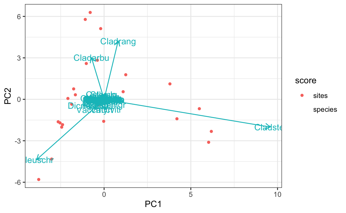
使用 autoplot()。

library(ggvegan)

## 载入需要的程辑包：ggplot2

# 使用空白主题
theme_set(theme_bw())

# 一键绘图
autoplot(pca)

还可以使用 fortify() 将对象转变为 data.frame，然后再作图。

# 生成数据框
df.pca <- fortify(pca)

# 查看数据
knitr::kable(df.pca[1:5,1:5])

score	label	PC1	PC2	PC3
species	Callvulg	-0.1469634	0.3483315	-0.2505840
species	Empenigr	0.1645106	-0.3731965	-0.5543083
species	Rhodtome	-0.0678718	-0.0810708	-0.0646412
species	Vaccmyrt	-0.5428697	-0.7446016	0.1973452
species	Vaccviti	0.0901303	-0.7247759	-0.6554941

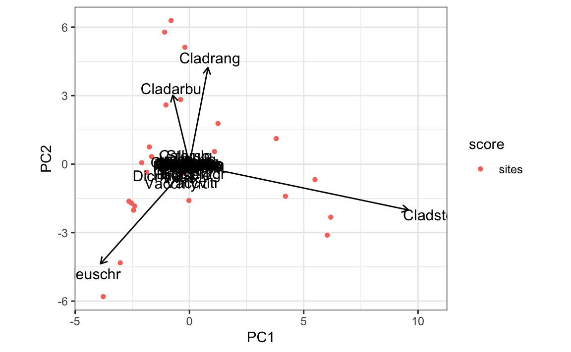
# 绘图
require(dplyr)

## 载入需要的程辑包：dplyr

## 
## 载入程辑包：'dplyr'

## The following objects are masked from 'package:stats':
## 
##     filter, lag

## The following objects are masked from 'package:base':
## 
##     intersect, setdiff, setequal, union

ggplot(mapping=aes(PC1,PC2,shape=score,color=score)) +
  geom_point(data=dplyr::filter(df.pca,score=="sites")) +
  geom_segment(data=dplyr::filter(df.pca,score=="species"),
               mapping = aes(x=0,y=0,xend=PC1,yend=PC2),
               arrow = arrow(length = unit(0.1,"inches")),show.legend = F) +
  geom_text(mapping = aes(PC1,PC2,label=label),data=filter(df.pca,score=="species"),show.legend = F)

除了PCA分析，ggvegan还顺便支持了CCA，RDA，metaMDS等vegan的分析结果。